Scottish Marine and Freshwater Science Volume 5 Number 10: Updating Fisheries Sensitivity Maps in British Waters
The requirement to display sensitive areas relating to the life history of commercially important fish species in British waters is well recognized and has been used by the Oil and Gas and other offshore industries for over thirty years. An update of thes
6 Technical Annex
6.1 Variable importance
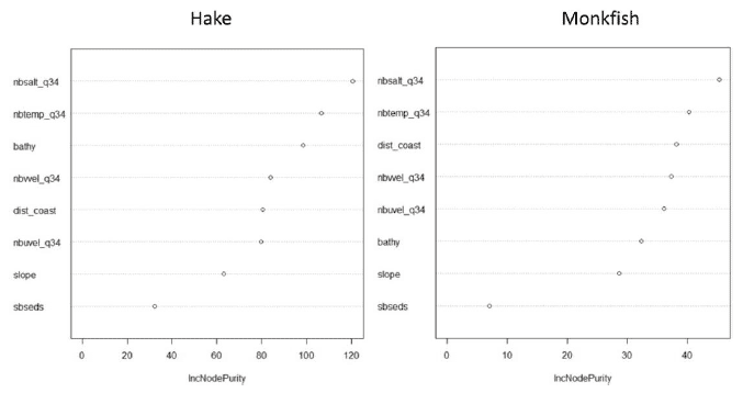
The variable importance in Random Forest is calculated using data "out of the bag". According to random sampling of observations, regardless whether with or without replacement, a certain percentage of the observations are not used for any individual tree (Gromping et al. 2010), that is, they are "out of the bag" ( OOB). The accuracy of a Random Forest prediction can be estimated from these OOB data and in the same way the variable importance can be estimated by quantifying how important the accuracy loss is after permuting this variable (see Gromping et al. 2010 for a more detailed explanation). The importance of the variables included in the Random Forest models was calculated and it is shown in Figures A1 to A3.
Figure A1: Relative importance of predictor variables used for the 0 group aggregations models of six demersal species. Bathy = Bathymetry, dist_coast = Distance to coast, nbsalt_q34 = Salinity near bottom, nbtemp_q34 = Temperature near bottom, nbuvel_q34 = Near bottom W-E current speed, nbvvel_q34 = Near bottom N-S current speed, sbseds = Sediment type and slope = slope.
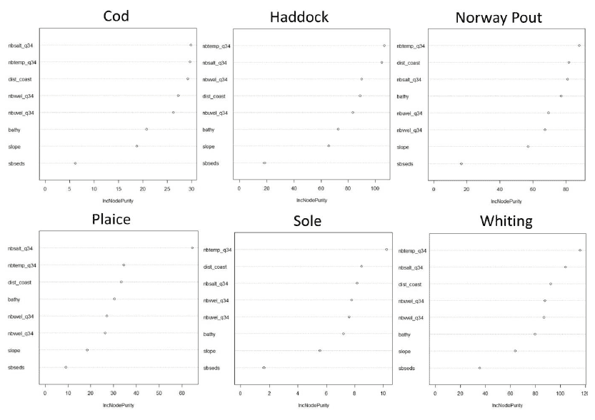
Figure A2: Relative importance of predictor variables used for the 0 group aggregations models of five pelagic species. Bathy = Bathymetry, dist_coast = Distance to coast, mdsalt_q34 = Salinity in mid-water, mdtemp_q34 = Temperature in mid-water, mduvel_q34 = mid-water W-E current speed, mdvvel_q34 = mid-water N-S current speed, sbseds = Sediment type and slope = slope.
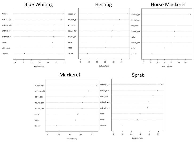
Figure A3: Relative importance of predictor variables used for the 0 group presence models for hake and monkfish (anglerfish).
6.2 Partial plots
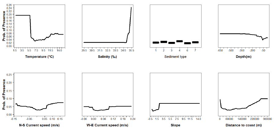
The partial dependence is the dependence of the probability of presence on one predictor variable after averaging out the effects of the other predictor variables in the model. This partial dependence can be plotted for different levels of each variable to show the specific effect of this variable in the probability of presence (partial plots). The partial plots for the thirteen species modelled (cod, haddock, Norway pout, plaice, sole, whiting, blue whiting, herring, horse mackerel, mackerel, sprat, hake and anglerfish) are shown in Figures A4- A16.
Figure A4: Partial plots from the cod 0 group aggregations model.
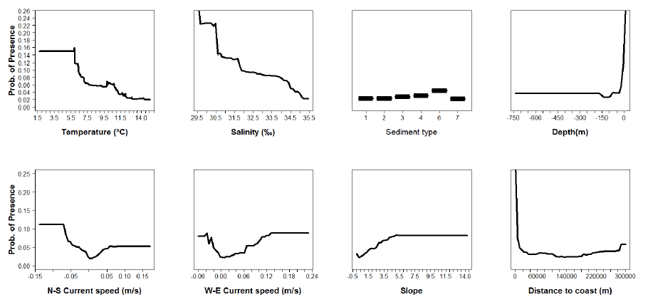
Figure A5: Partial plots from the haddock 0 group aggregations model.
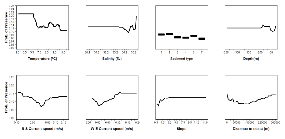
Figure A6: Partial plots from the Norway pout 0 group aggregations model .
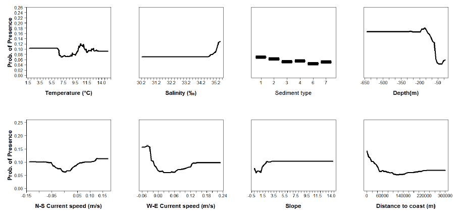
Figure A7: Partial plots from the plaice 0 group aggregations model.
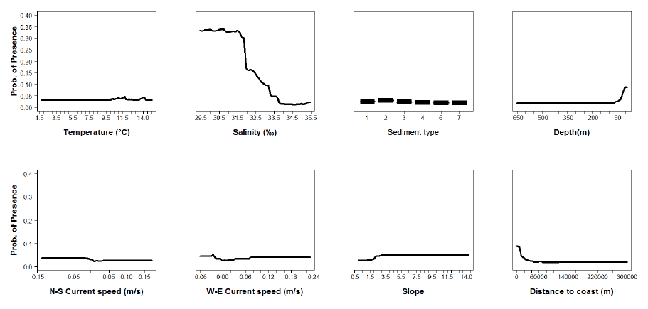
Figure A8: Partial plots from the sole 0 group aggregations model.
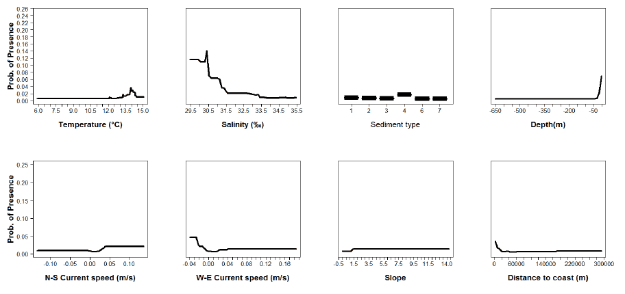
Figure A9: Partial plots from the whiting 0 group aggregations model.
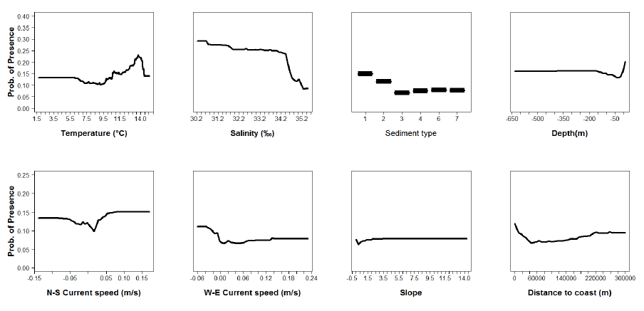
Figure A10: Partial plots from the blue whiting 0 group aggregations model.
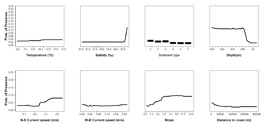
Figure A11: Partial plots from the herring 0 group aggregations model.
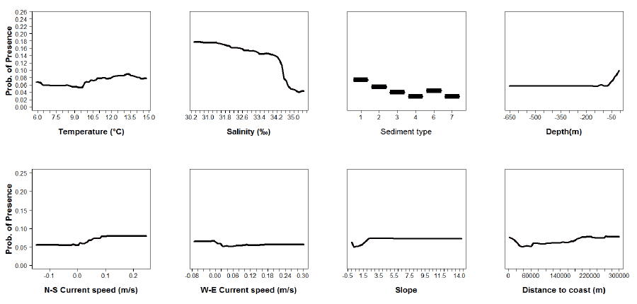
Figure A12: Partial plots from the horse mackerel 0 group aggregations model.
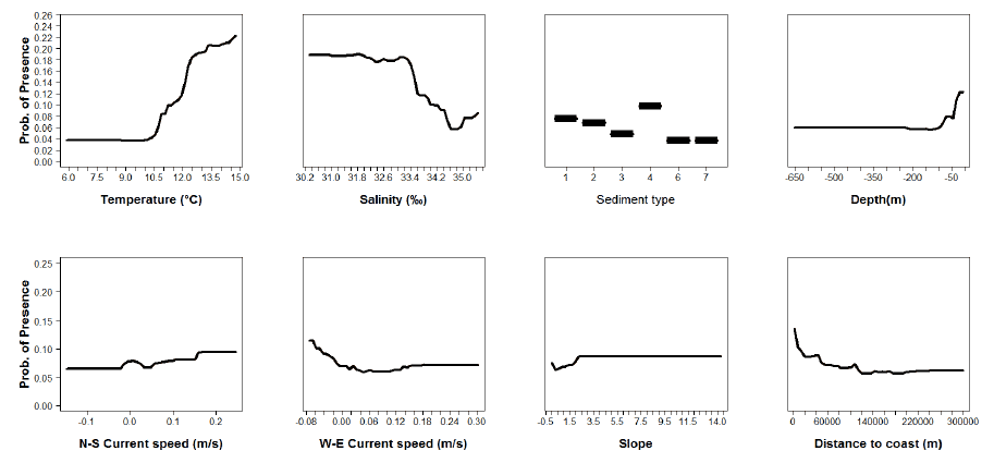
Figure A13: Partial plots from the mackerel 0 group aggregations model.
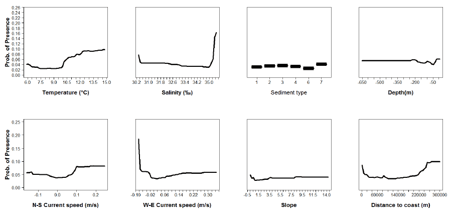
Figure A14: Partial plots from the sprat 0 group aggregations model.
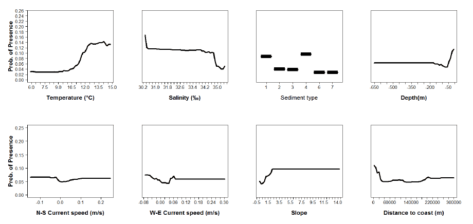
Figure A15: Partial plots from the hake 0 group presence-absence model.
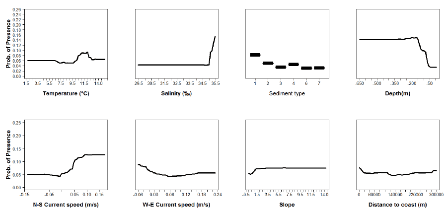
Figure A16: Partial plots from the anglerfish 0 group presence-absence model.
Contact
There is a problem
Thanks for your feedback